How Long Will It Take? – Part 2 – So, Does It Work?
After writing the original How Long Will It Take? post, I kept wondering how to measure if the estimation method described therein (from here on referred to as “Historical Lead Time”, or HLT) is effective, for some definition of effective. What I realized is, since the estimation method does not require human input, I could use historical data and simulate what the method would estimate at any particular point in time. This blog post describes this experiment and demonstrates a very surprising finding.
TL;DR: It turns out that the HLT method minimizes estimation error better than every other tested method except one, which is… *drumroll*… “pick the average so far” as the estimate. Read below for details and caveats. Also, it would be very helpful to run this experiment on many data sets instead of just the one I used, please contact me if you can provide a data set to run this experiment on.
Experiment Objective
Determine usefulness of estimating software work using percentile estimates based solely on observed past data as described in How Long Will It Take? .
Experiment Hypothesis
HLT estimates are better than random estimates. (Spoiler: they are! … or more correctly: experiment results do not refute this hypothesis)
Experiment Metric
Sum of square error, which will be the difference between estimated duration and actual work item duration, squared.
Experiment Design
The experiment is a simulation of what would the estimates be at specific times in the past. Given a data set of work start and stop times, simulation starts after completion of first work item and ends after completion of last work item in the data set.
Experiment uses multiple estimation models. The model with the least cumulative sum of square error is deemed the best. Where appropriate, models are tracked per 25th, 50th, 75th, 90th, 95th, and 99th percentiles. Models used in the experiment are:
- HLT: Estimation method described in How Long Will It Take?.
- Levy: Estimation method that assumes distribution of observed work item durations can be described as a Levy distribution. This model is included to showcase a terrible model.
- Gaussian: Estimation method that assumes distribution of observed work item durations can be described as a Gaussian/Normal distribution. This model is included to showcase a “dumb” model as a sanity check.
- Random: Estimation method that simply picks a random number between zero and longest duration observed so far. This model is included to provide a baseline to compare against.
- Weibull: Estimation method that assumes distribution of observed work item durations can be described as a Weibull distribution. This model is included because it is seems to be the go-to model used by people who take estimation seriously.
In addition to the above models, each model is also tested with and without sample bootstrap to a sample size of 1000, as described in How Long Will It Take?
Data set used for the experiment is Data Set 1, consisting of 150 work item start and stop times.
Each simulation is performed using the following procedure:
- Using Data Set 1, create a timeline of start and stop events to playback.
- Playback the timeline created in 1.
- Upon observing a work item start event, notify the estimation model of work item start. If the model can generate an estimate (model must observe two completed work items prior to generating an estimate), compare the generated estimate with actual known duration, calculate the square error, and record it.
- Upon observing a work item stop event, notify the estimation model of work item stop.
- Continue playback until the timeline is exhausted.
Experiment Results
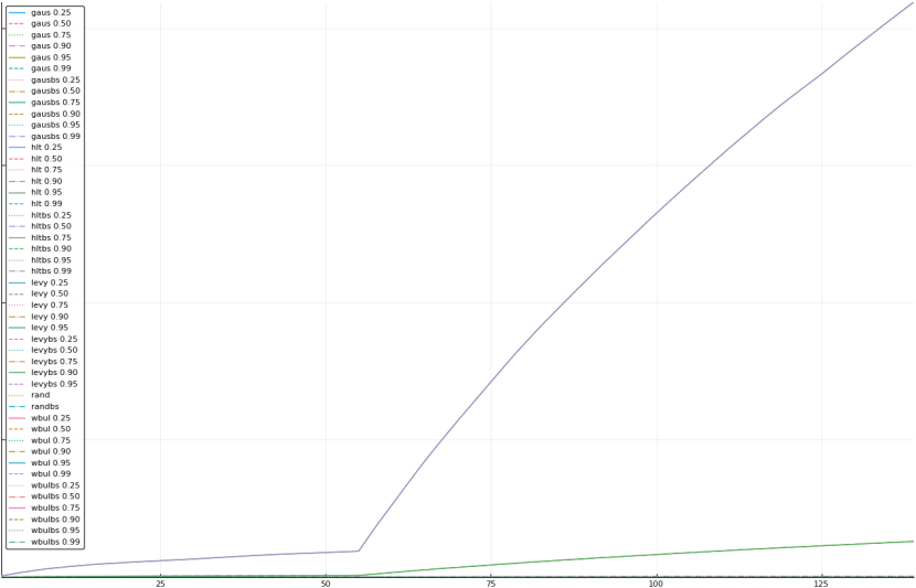
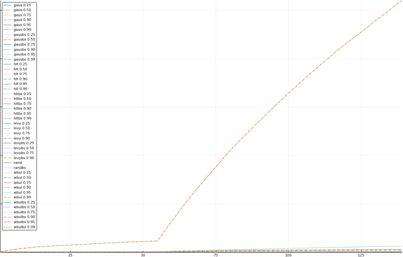
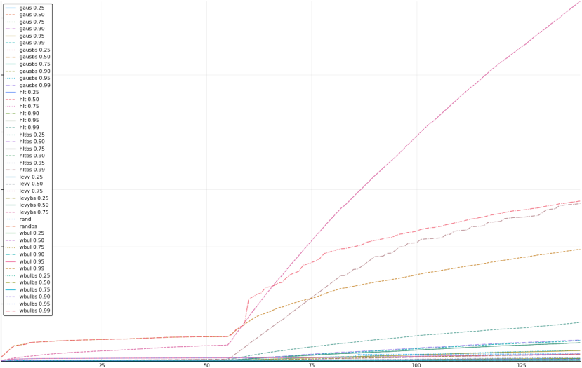
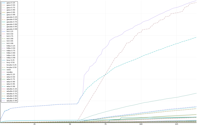
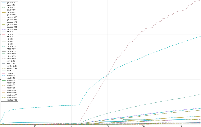
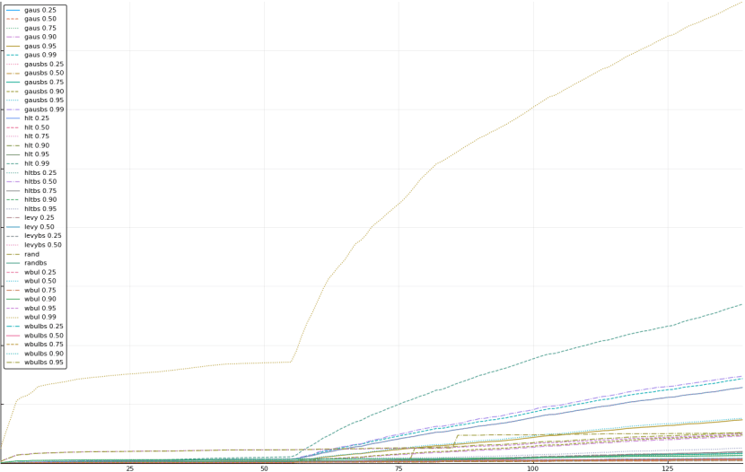
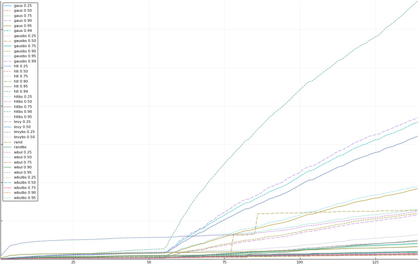
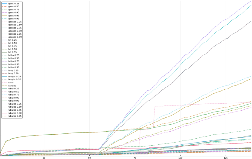
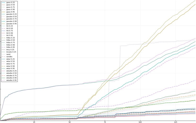
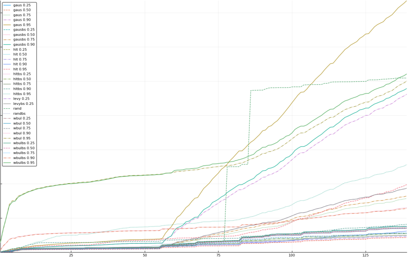
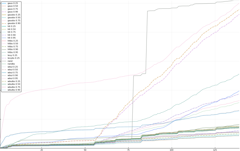
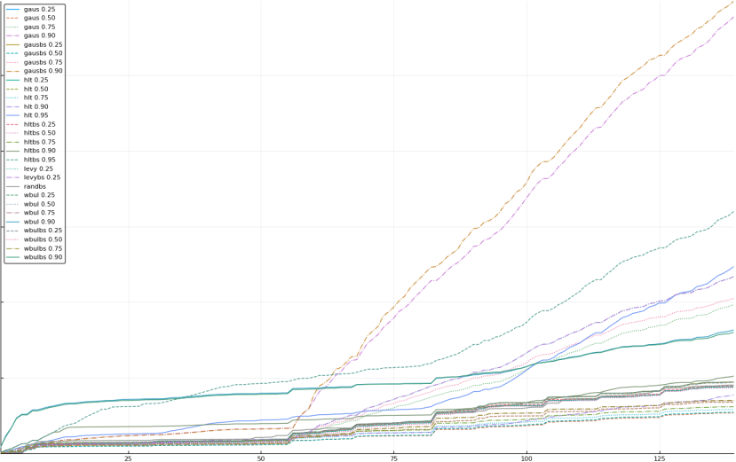
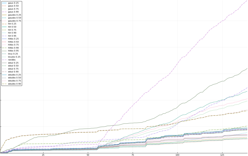
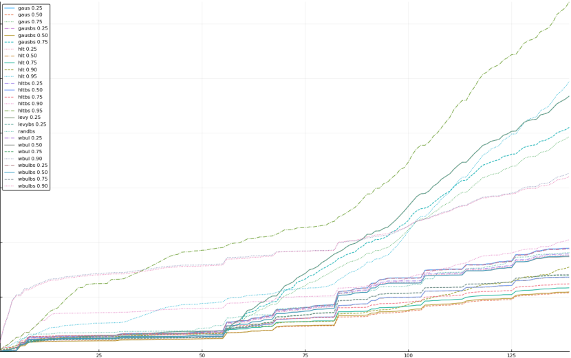
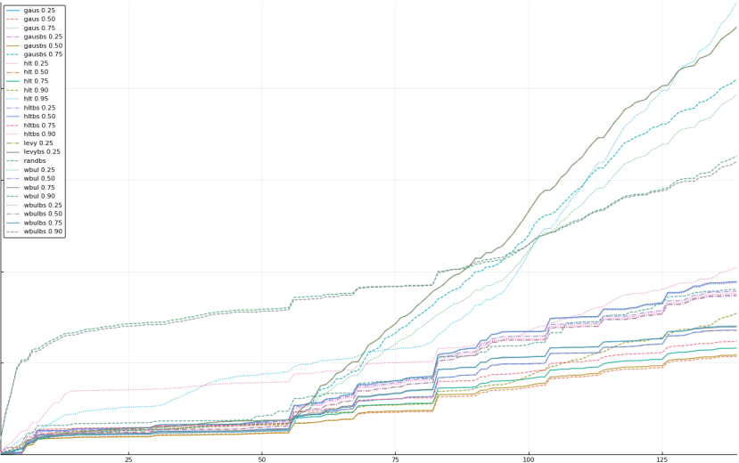
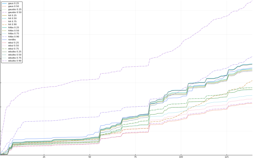
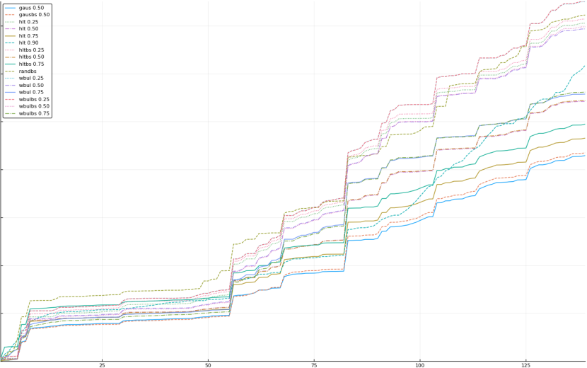
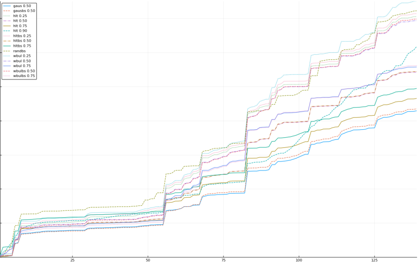
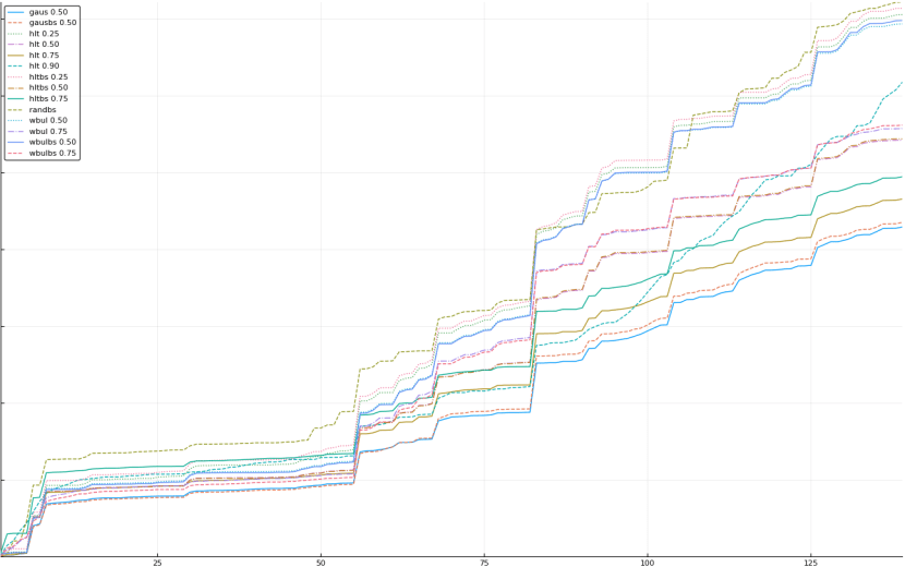
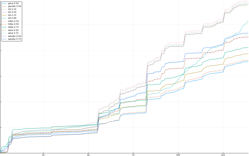
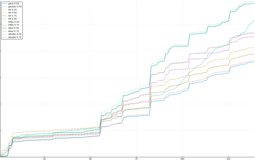
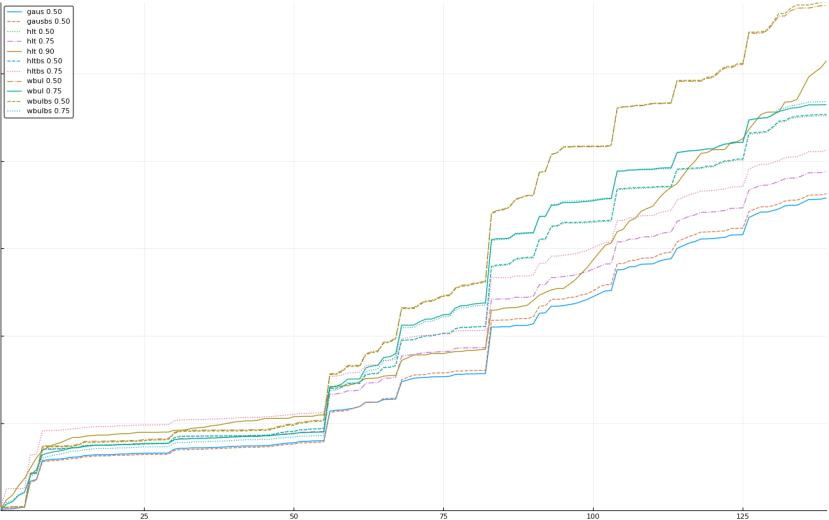
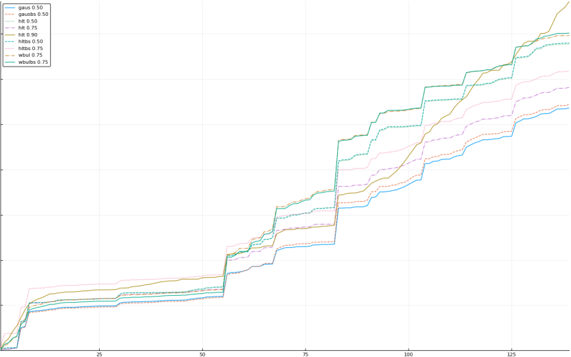
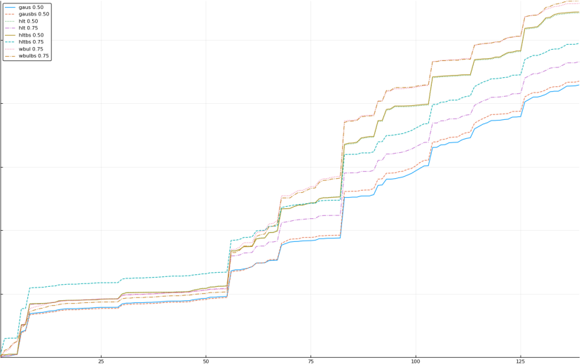
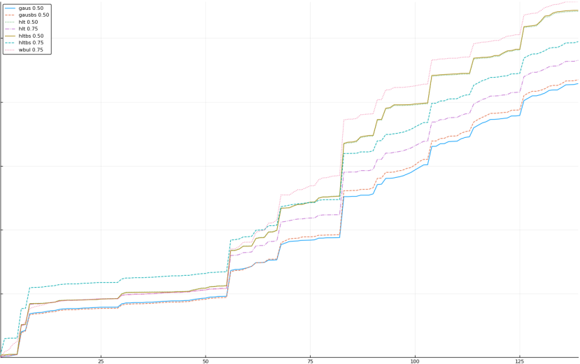
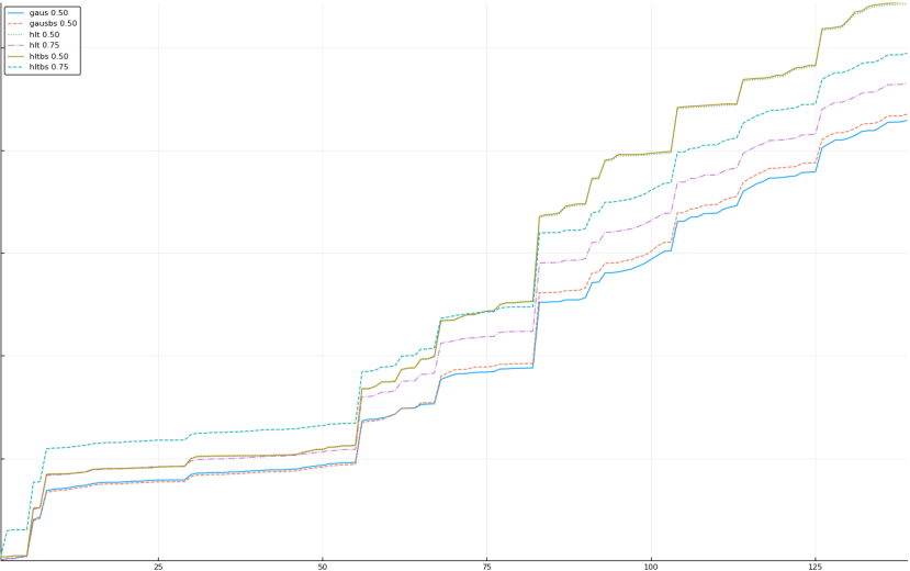
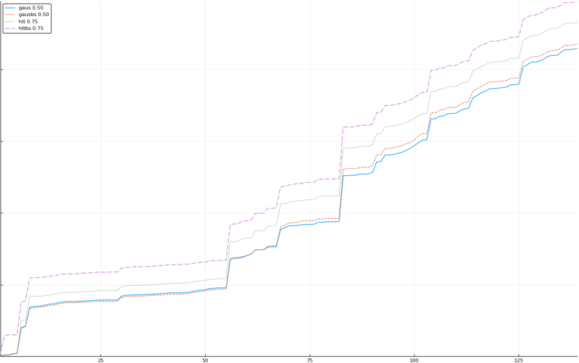
A rich way to demonstrate the results is to plot the cumulative sum of square error for each model and each percentile together (model+percentile, e.g.: “levy 0.99”, means Levy model 99th percentile, “hltbs 0.75”, means HLT model with bootstrapped sample at 75th percentile). These plots are included below. In consecutive plots, the worse performing model+percentile line is eliminated so that we can see more detail regarding better performing models. Also, the shape of error accumulation is instructive. The elimination order is (from most accumulated error to least accumulated error):
levy 0.99, levybs 0.99, levy 0.95, levybs 0.95, levy 0.90, levybs 0.90, levy 0.75, levybs 0.75, wbulbs 0.99, hltbs 0.99, wbul 0.99, hlt 0.99, gausbs 0.99, gaus 0.99, levy 0.50, levybs 0.50, gausbs 0.95, gaus 0.95, wbulbs 0.95, rand, wbul 0.95, gausbs 0.90, gaus 0.90, hltbs 0.95, hlt 0.95, levy 0.25, levybs 0.25, gausbs 0.75, gaus 0.75, wbul 0.90, wbulbs 0.90, hltbs 0.90, gaus 0.25, gausbs 0.25, wbulbs 0.25, wbul 0.25, randbs, hltbs 0.25, hlt 0.25, wbulbs 0.50, wbul 0.50, hlt 0.90, wbulbs 0.75, wbul 0.75, hltbs 0.50, hlt 0.50, hltbs 0.75, hlt 0.75, gausbs 0.50, gaus 0.50
Here is a list that performed worse than “rand”:
levy 0.99, levybs 0.99, levy 0.95, levybs 0.95, levy 0.90, levybs 0.90, levy 0.75, levybs 0.75, wbulbs 0.99, hltbs 0.99, wbul 0.99, hlt 0.99, gausbs 0.99, gaus 0.99, levy 0.50, levybs 0.50, gausbs 0.95, gaus 0.95, wbulbs 0.95
Here is a list that performed worse than “randbs”:
levy 0.99, levybs 0.99, levy 0.95, levybs 0.95, levy 0.90, levybs 0.90, levy 0.75, levybs 0.75, wbulbs 0.99, hltbs 0.99, wbul 0.99, hlt 0.99, gausbs 0.99, gaus 0.99, levy 0.50, levybs 0.50, gausbs 0.95, gaus 0.95, wbulbs 0.95, rand, wbul 0.95, gausbs 0.90, gaus 0.90, hltbs 0.95, hlt 0.95, levy 0.25, levybs 0.25, gausbs 0.75, gaus 0.75, wbul 0.90, wbulbs 0.90, hltbs 0.90, gaus 0.25, gausbs 0.25, wbulbs 0.25, wbul 0.25
Here is a list that performed better than “randbs”:
hltbs 0.25, hlt 0.25, wbulbs 0.50, wbul 0.50, hlt 0.90, wbulbs 0.75, wbul 0.75, hltbs 0.50, hlt 0.50, hltbs 0.75, hlt 0.75, gausbs 0.50, gaus 0.50
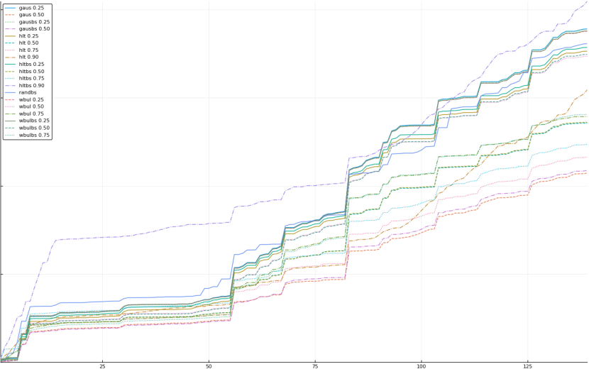
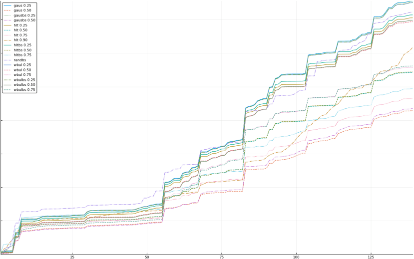
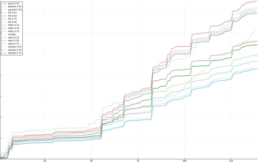
The vertical axis is the accumulated square error with units and values omitted as relative comparison is sufficient. The horizontal axis is enumerating estimates from first to last. Note that the same line style and line color does not represent the same model+percentile from plot to plot. Refer to the legend for identification of model and percentile.
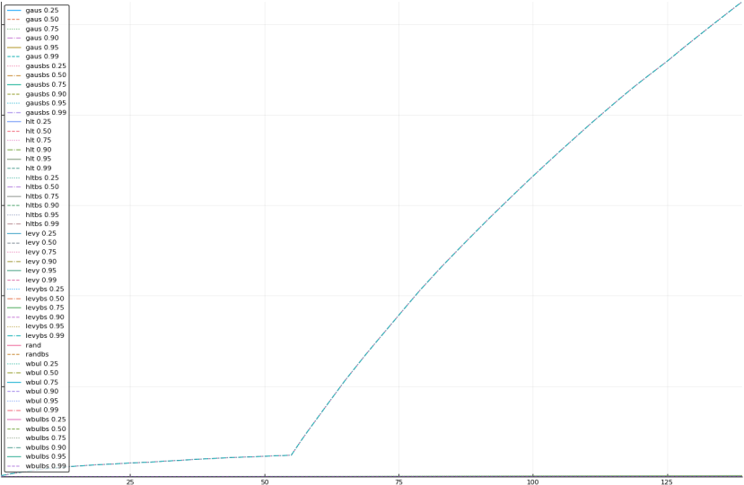
All models and percentiles
Eliminated levy 0.99 and levybs 0.99
Eliminated levy 0.95 and levybs 0.95
Eliminated levy 0.90 and levybs 0.90
Eliminated levy 0.75 and levybs 0.75
Eliminated wbulbs 0.99
Eliminated hltbs 0.99
Eliminated wbul 0.99
Eliminated hlt 0.99
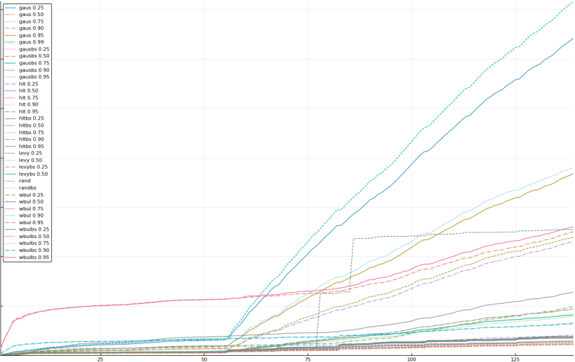
Eliminated gausbs 0.99
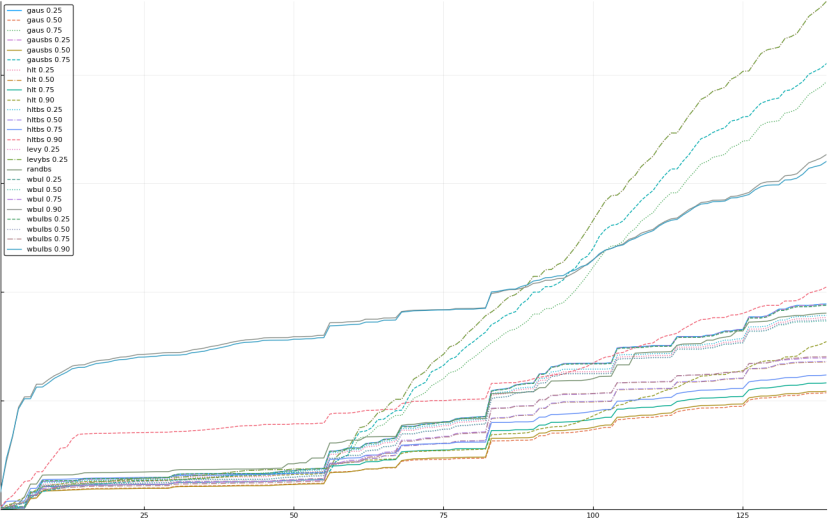
Eliminated levy 0.50 and levybs 0.50
Eliminated gausbs 0.95

Eliminated gaus 0.95
Eliminated wbulbs 0.95

Eliminated rand (displayed are all experiments that performed better than rand)
Eliminated wbul 0.95
Eliminated gausbs 0.90
Eliminated gaus 0.90
Eliminated hltbs 0.95
Eliminated hlt 0.95
Eliminated levy 0.25
Eliminated levybs 0.25

Eliminated gausbs 0.75

Eliminated gaus 0.75
Eliminated wbul 0.90
Eliminated wbulbs 0.90
Eliminated hltbs 0.90
Eliminated gaus 0.25
Eliminated gausbs 0.25
Eliminated wbulbs 0.25
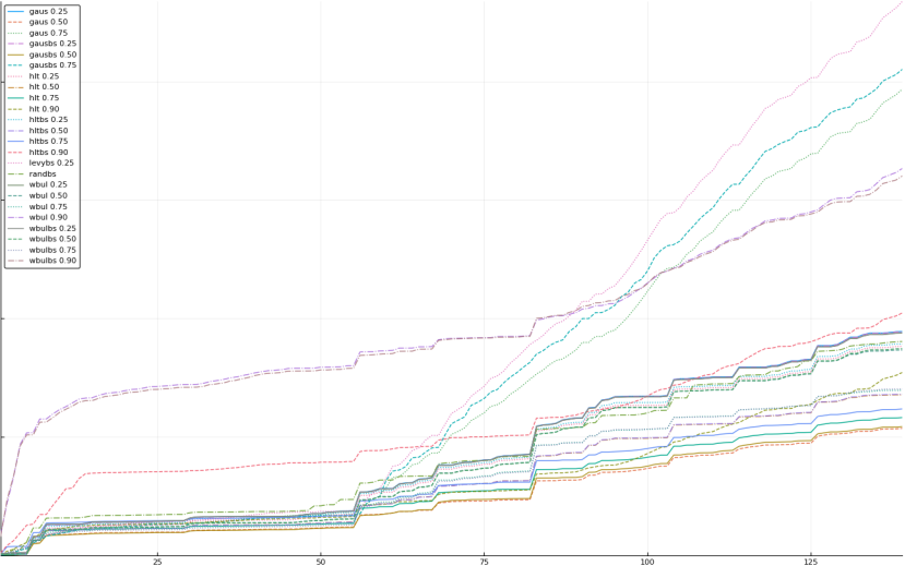
Eliminated wbul 0.25
Eliminated randbs (displayed are all experiments that performed better than randbs)
Eliminated hltbs 0.25
Eliminated hlt 0.25
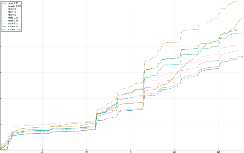
Eliminated wbulbs 0.50
Eliminated wbul 0.50
Eliminated hlt 0.90
Eliminated wbulbs 0.75
Eliminated wbul 0.75
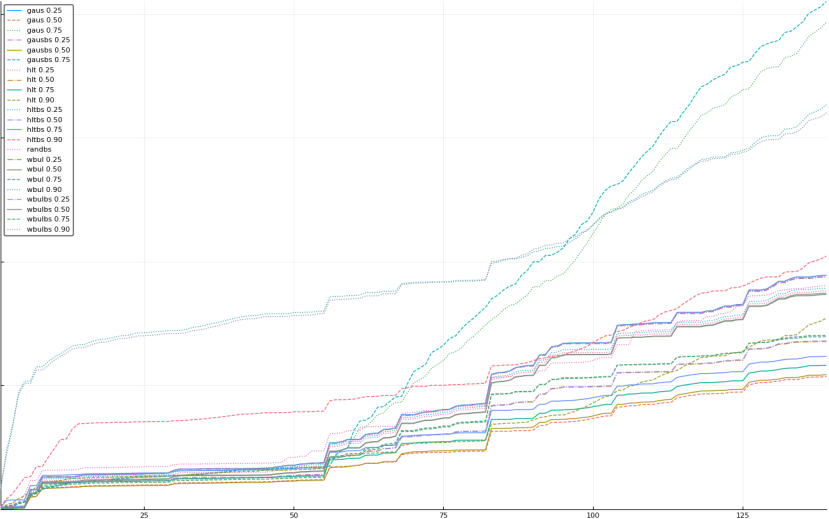
Eliminated hltbs 0.50 and hlt 0.50
Experiment Analysis
Main concern is that experimental data is only one data set of 150 items. While the results are surprising, they may not be typical. I need other data sets to run this experiment on (please get in touch if you’re interested in testing your data set).
Regarding accuracy, the fitting of Levy distribution was fairly unsophisticated (calculate mean and variance of sample and use that to generate a Levy distribution). I didn’t expect Levy to perform well and as it was just background to testing the main hypothesis, I didn’t bother implementing a more sophisticated distribution fitting. Weibull distribution, on the other hand, is a pretty good fit as it uses least-squares fit to observed distribution. In summary, Levy distribution fit is crap, Weibull distribution fit should be pretty good. Gaussian distribution fit is straightforward, so it should also be good.
It is interesting to see the impact of outliers on estimation method (large spikes in error graphs). While an outlier destroys some estimators (one can observe points in the graphs where estimator makes a turn for the worse and rapidly departs from best performer), other estimators seem to be robust to outliers. Note that model may be robust or not depending on which percentile is used for estimation.
Another thing of note is that the best performing percentiles are 50th and 75th and not others. This attraction toward the average was a surprise.
Why does “pick the average so far” (more precisely, pick 50th percentile of estimated normal distribution from observed data without bootstrapping) work so well? I assume that part of it is due to normal distribution being robust to outliers, especially once there is enough data to anchor the distribution away from the outlier pretty well. I’m not sure why HLT 75th percentile is better than HLT 50th though.
Bootstrapped random estimator (rndmbs) performed really well, and it also has the same shape as the winning estimators. Note that rndmbs used the same random seed as rndm to select a number between zero and maximum in the sample. What most likely happened is the interplay between bootstrapping process (sampling with replacement) and random estimate being a random number between zero and maximum in the sample. Early on, before the outlier, bootstrapping did not change the maximum, and random estimators chose the same number up to the same maximum. Once an outlier occurred, we see that rndm selected it at least twice. However, it may be the case that the bootstrapping process for rndmbs did not pick the outlier into the bootstrapped sample, allowing rndmbs to pick from a smaller numeric range. From the plot of rndm, it looks like rndmbs only had to get lucky like this twice.
Experiment Learnings
It seems that in order to minimize error in estimates, the best thing to do is pick an estimator robust to outliers. In particular, the best (according to this data set), is to estimate a normal distribution from observed data and pick the mean. If this holds for other data sets, it means that we can all let go fancy statistical methods and use this very simple “pick the average” approach from now on. Imagine how much simpler our estimating lives could be ;).
Questions For The Future
Do these patterns hold for other data sets? If you have a data set, please get in touch.
The experiment only checks the estimation at the start of work (typically when we do estimation), but this doesn’t take into account the full HLT technique of continuous estimation. How good would these estimators be in a continuous (for example, once a day) estimation?
The experiment does not check if models get better at estimation as time progresses. This may be interesting to see.
Typically, when we estimate, the impact of finishing early and finishing late is asymmetric. What would be the results under different penalties for having estimates that are too optimistic (work actually takes longer than estimate).
What is the impact of choosing different seeds for bootstrapping as well as different seeds for estimators using random?
